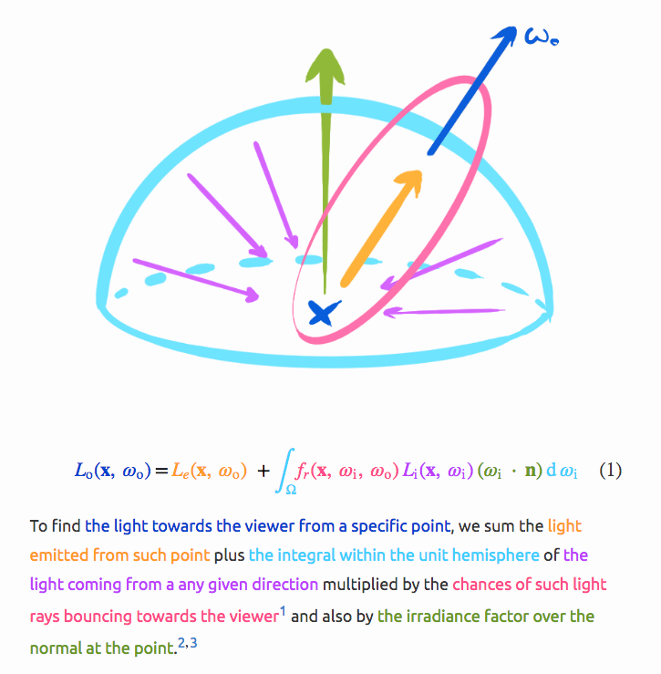
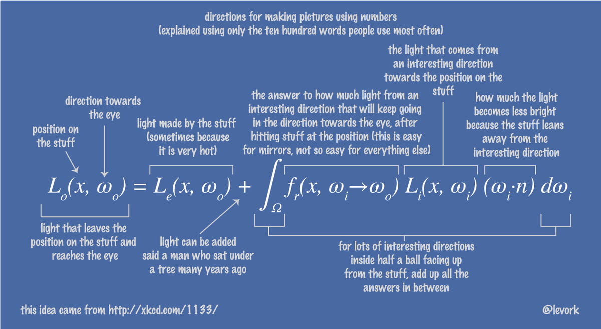
The rendering equation aims to describe what the light distribution for a specific scene is, under several assumptions. The most important assumption is that we are working in a geometrical optics framework - so we do not consider the wave properties of light - meaning no diffraction for example, we also do not consider quantum effects, such as phosphorescence. If the rendering equation is not in its spectral form, then there's also no dispersion.
There are additional constraints on top of what we have for geometrical optics, like light travels instantaneously, light rays traveling in straight paths from surface to surface (no spatially continuously varying indices of refraction), no polarization, etc. Many of the constraints can be removed in more general formulations (which are also available), but usually that incurs heavier computations.
So the rendering equation serves as an approximation to how light works in the real world, but since we want to model only a subset of light effects, various simplification are made in order to make the problem easier to solve.
Let us consider the commonly shown formulation:


The above images are linked from: Raytracing - Rendering Equation Insight
I believe these images are fairly self-explanatory. The function $f_r$ referred to as the BRDF (or more generally the BSDF) describes the interaction of materials with light. Often in real-time graphics this is referred to as the illumination or reflectance model - one such example is the Blinn–Phong reflection model, there is the Cook-Torrance model too, and several others. All of those are brdfs/bsdfs, or constituent parts of brdfs/bsdfs.
Flat, Gouraud, and Phong shading (or more correctly Gouraud and Phong interpolation) is really referring to how the normals of a model are treated (interpolated).
Flat shading simply uses the actual normals of an object. If we could render objects made up of infinitely many triangles, even flat shading would be ideal. However, as for most things in graphics, efficiency is key, so we cannot use infinitely may triangles. For that reason people have chosen to modify the surface normals of objects, in order to get a smoother appearance - as if they used a lot more triangles. How is this achieved? Well, one can find per-vertex normals, that are a weighted sum of the face normals, so that a smooth like appearance is achieved. For example by using approaches such as the one described in the following publication: Weights for Computing Vertex Normals from Facet Normals.
Gouraud shading (Gouraud interpolation), refers to computing the illumination per vertex, using these normals, and then interpolating the resulting color over the triangle - this explains why it has discontinuities at edges and vertices.
Phong shading (Phong interpolation) interpolates the normals over the triangle (by using barycentric coordinates) and then computes the shading using those per-pixel which results in an overall smoother appearance. Note that discontinuities at the outline of the object can still be visible - this modifies only the shading of the object, and not its actual geometry.
One can go further and use bump mapping, derivative mapping, or normal mapping, in order to further enrich the shading information over an otherwise flat surface, by modifying the normals.
All of those normal modifications (Gouraud and Phong interpolation; bump, derivative, and normal mapping) produce normals which are commonly referred to as shading normals. Note that those violate energy conservation principles in general, and may cause various artifacts. But obviously this is the trade-off for performance. So all of those techniques fall under the umbrella of normals modification and are not illumination models in their own right (but those normals are used in the brdf and the rendering equation to compute shading - where the shading part in the terms goes - I still believe interpolating is a better naming).
To understand the shadow conundrum, let's look at the solution of the rendering equation. The rendering equation in mathematics is known as a Fredholm integral equation of the second kind, under some assumptions, its solution is given through the sum of increasingly dimensional integrals: Liouville–Neumann series. I will avoid writing out the integrals explicitly, since it will get ugly very quickly, you can find the expansion in Veach's thesis however. I will just use the operator formulation of the rendering equation. Let $L = L_o$, and $T$ be that integral from the images. Then the rendering equation can be written concisely as:
$$L = L_e + L_r = L_e + TL$$
$$L-TL = L_e$$
$$(I-T)L = L_e$$
$$L = (I-T)^{-1}L_e = \sum_{k=0}^{\infty}T^kL_e$$
The last equality holds due to the Liouville-Neumann expansion that I talked about. This is a sum of increasingly dimensional integrals similar to the one you had in the rendering equation (with a few additions) - usually this is also done with respect to the area formulation of the rendering equation (the images here provide the solid angle formulation). Informally $T^k$ means that there were $k$ bounces before reaching the light source, so it's a sum of the energy coming from paths starting at the eye and ending at a light source, of length $1, 2, 3, ..., \infty$. Let's look at the area formulation of the rendering equation:
$$L(\pmb{x}_0\leftarrow\pmb{x}_1) = L_e(\pmb{x}_0\leftarrow\pmb{x}_1) + \\ \int_{\mathcal{M}}f_r(\pmb{x}_0\leftarrow\pmb{x}_1\leftarrow\pmb{x}_2)L(\pmb{x}_1\leftarrow\pmb{x}_2)\frac{\cos\theta_{\pmb{x}_1}\cos\theta_{\pmb{x}_2}}{\|\pmb{x}_2-\pmb{x}_1\|^2_2}V(\pmb{x}_1,\pmb{x}_2)\,d\pmb{x}_2$$
Here $\mathcal{M}$ is the set of all surface points of the scene (including lights), $L(\pmb{x}_0\leftarrow\pmb{x}_1)$ gives you the radiance traveling from surface point $\pmb{x}_1$ to $\pmb{x}_0$, $L_e(\pmb{x}_0\leftarrow\pmb{x}_1)$ gives you the emission from $\pmb{x}_1$ towards $\pmb{x}_0$. To relate the brds to the previous formulation, one can set: $\omega_o = \frac{\pmb{x}_0-\pmb{x}_1}{\|\pmb{x}_0-\pmb{x}_1\|}$, $\omega_i = \frac{\pmb{x}_2-\pmb{x}_1}{\|\pmb{x}_2-\pmb{x}_1\|}$, and $\pmb{x} = \pmb{x}_1$. Furthermore, $\cos\theta_{\pmb{x}_1} = \omega_i \cdot \pmb{n}$, where $\pmb{n}$ is the surface normal at $\pmb{x}_1$, similarly $\cos\theta_{\pmb{x}_2} = -\omega_i \cdot \pmb{n}_{\pmb{x}_2}$, where $\pmb{n}_{\pmb{x}_2}$ is the surface normal at $\pmb{x}_2$. The squared Euclidean distance in the denominator is due to the inverse-square law (it's implicitly encoded in the solid angle formulation). Finally, $V(\pmb{x}_1,\pmb{x}_2)$ is the visibility function - it is equal to $1$ if there is nothing between $\pmb{x}_1$ and $\pmb{x}_2$ (no occlusion), and $0$ otherwise (it is also implicit in the solid angle formulation) - this is the function that encodes shadows. Approximations, that do not produce shadows, have simply thrown away or modified that visibility function (one such modification is replacing $V$ with the ambient occlusion or with information from a shadow map). This is done for efficiency reasons once again, as instead you would have to trace a ray from $\pmb{x}_1$ to $\pmb{x}_2$ and intersect against the scene to check for occlusion.
Let us consider the simplifications that are usually made in real-time graphics. Most implementations, simply cut the Neumann sum to the 2nd term:
$$L = L_e + TL_e + T^2L_e + ... \approx L_e + TL_e$$
So anything beyond direct illumination and emission is thrown away. This has important implications - such as: no indirect illumination or scattering effects. Let's consider what this amounts to:
$$L = L_e + TL_e$$
$$L(\pmb{x}_0\leftarrow\pmb{x}_1) = L_e(\pmb{x}_0\leftarrow\pmb{x}_1) + \\ \int_{\mathcal{M}}f_r(\pmb{x}_0\leftarrow\pmb{x}_1\leftarrow\pmb{x}_2)L_e(\pmb{x}_1\leftarrow\pmb{x}_2)\frac{\cos\theta_{\pmb{x}_1}\cos\theta_{\pmb{x}_2}}{\|\pmb{x}_2-\pmb{x}_1\|^2_2}V(\pmb{x}_1,\pmb{x}_2)\,d\pmb{x}_2$$
There is one small difference compared to the area formulation, and that is the fact that we have $L_e$ in the integral and not $L$, so it is not a recursive integral anymore. It is still an integral however, which implies an infinite sum - this is currently not very fast to compute, unless you have specialized hardware like RTX, especially for more complex scenes. Note that the integral is over all surface points emitting light, so you would in general need to sum up the light coming from area lights, skyboxes etc.
So the next simplification that is usually done, is using point lights. Point lights have the computationally efficient property, that they are represented through Dirac delta functions. A Dirac delta function, essentially allows you to get rid of the integral - the light comes only from a single direction. Then your integral turns into a finite sum over all point lights in the scene (a similar argument may be made for directional or spot lights, note that the light cosine term disappears, since informally there's no normal to speak of):
$$L(\pmb{x}_0\leftarrow\pmb{x}_1) = L_e(\pmb{x}_0\leftarrow\pmb{x}_1) + \\ \sum_{k=1}^{N}f_r(\pmb{x}_0\leftarrow\pmb{x}_1\leftarrow\pmb{y}_k)L_k(\pmb{x}_1\leftarrow\pmb{y}_k)\frac{\cos\theta_{\pmb{x}_1}}{\|\pmb{y}_k-\pmb{x}_1\|^2_2}V(\pmb{x}_1,\pmb{y}_k)$$
Where $L_e$ is generally constant, $L_k$ is the radiance of light source $k$ and $\pmb{y}_k$ is the position of light source $k$. If your material is diffuse then $f_r$ and the radiance of the point light do not change with directions, then $L_i$ and $f_r$ are also constant so you get the (possibly) familiar expression:
$$L = L_e + \sum_{k=1}^{N}f_rL_k\cos\theta_k V(\pmb{x}_1,\pmb{y}_k)$$
$$color = emission + \sum_{k=1}^{N}ObjectColor * LightColor * \cos\theta_k * VisibilityFromLight\_k$$
The only thing that is usually not there is the $V$ term, since it requires tracing rays through the scene, which standard rasterization algorithms don't do. So it's either set to $1$, or replaced with information from a shadow map (for each summand the shadow map from this light's perspective ought to be used for semi-correct results). Often times the remaining terms that were cut off $T^2L_e + T^3L_e + ... + T^{\infty}L_e$ are substituted with a constant ambient light term or with an ambient occlusion term.
Path tracing usually solves the rendering equation without any of the above simplifications (but requires a lot more computational power), that is the reason why images produced by it look so realistic.
Whole books may be written on this matter. But I hope I managed to clarify at least some things regarding Gouraud, Phong interpolation, shadows, and how all of this ties into the rendering equation.

