-- Sorry for the long post, but I prefer to do that way because "Devil is in the details." :)
I am writing a path tracer from the scratch and it is working nicely for perfectly diffuse (Lambertian) surfaces (i.e. the furnace test indicates - at least visually - that it is energy conserving, and rendered images match those generated with Mitsuba renderer for the same parameters). Now I am implementing the support for the specular term of the original Cook-Torrance microfacet model, in order to render some metallic surfaces. However, it seems that this BRDF is reflecting more energy than that received. See the example images below:
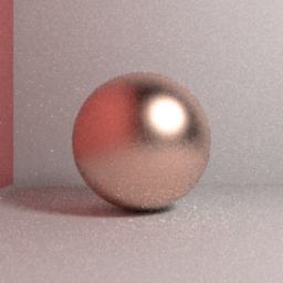
Above image: Mitsuba reference (assumed to be correct) image: Path tracing with direct light sampling, importance hemisphere sampling, max path lenght = 5, 32 stratified spp, box filter, surface roughness = 0.2, RGB.
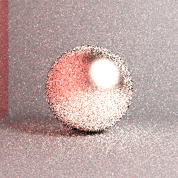
Above image: Actual rendered image: Brute force naïve path tracing, uniform hemisphere sampling, max path lenght = 5, 4096 stratified spp, box filter, surface roughness = 0.2, RGB. Despite some differences with respect to the rendering settings, it is clear that the rendered image will not converge to the reference shown before.
I tend to think that it is not an implementation problem, but an issue regarding the proper use of the Cook-Torrance model within the rendering equation framework. Below I explain how I am evaluating the specular BRDF and I would like to know if I am doing it properly and, if not, why.
Before going into the nitty-gritty details, notice that the renderer is quite simple: 1) implements only the brute force naïve path tracing algorithm - no direct light sampling, no bi-directional path tracing, no MLT; 2) all sampling is uniform on the hemisphere above the intersection point - no importance sampling at all, neither for diffuse surfaces; 3) the ray path has a fixed maximum length of 5 - no russian roulette; 4) radiance/reflectance is informed through RGB tuples - no spectral rendering.
Cook Torrance microfacet model
Now I will try to construct the path I've followed to implement the specular BRDF evaluation expression. Everything starts with the rendering equation $$ L_o(\textbf{p}, \mathbf{w_o}) = L_e + \int_{\Omega} L_i(\textbf{p}, \mathbf{w_i}) fr(\mathbf{w_o}, \mathbf{w_i}) \cos \theta d\omega $$ where $\textbf{p}$ is the intersection point at the surface, $\mathbf{w_o}$ is the viewing vector, $\mathbf{w_i}$ is the light vector, $L_o$ is the outgoing radiance along $\mathbf{w_o}$, $L_i$ is the radiance incident upon $\textbf{p}$ along $\mathbf{w_i}$ and $\cos \theta = \mathbf{n} \cdot \mathbf{w_i}$.
The above integral (i.e. the reflection term of the rendering equation) can be approximated with the following Monte Carlo estimator $$ \frac{1}{N} \sum_{k=1}^{N} \frac{ L_i(\textbf{p}, \mathbf{w_k}) fr(\mathbf{w_k}, w_o) \cos \theta }{p(\mathbf{w_k})} $$ where $p$ is the probability density function (PDF) that describes the distribution of the sampling vectors $\mathbf{w_k}$.
For actual rendering, the BRDF and PDF must be specified. In the case of the specular term of the Cook-Torrance model, I am using the following BRDF $$ fr(\mathbf{w_i}, \mathbf{w_o}) = \frac{DFG}{\pi (\mathbf{n} \cdot \mathbf{w_i})(\mathbf{n} \cdot \mathbf{w_o})} $$ where $$ D = \frac{1}{m^2 (\mathbf{n} \cdot \mathbf{h})^4} \exp \left( {\frac{(\mathbf{n} \cdot \mathbf{h})^2 - 1}{m^2 (\mathbf{n} \cdot \mathbf{h})^2}} \right) $$ $$ F = c_{spec} + (1 - c_{spec}) (1 - \mathbf{w_i} \cdot \mathbf{h})^5 $$ $$ G = \min \left( 1, \frac{2(\mathbf{n} \cdot \mathbf{h})(\mathbf{n} \cdot \mathbf{w_o})}{\mathbf{w_o} \cdot \mathbf{h}}, \frac{2(\mathbf{n} \cdot \mathbf{h})(\mathbf{n} \cdot \mathbf{w_i})}{\mathbf{w_o} \cdot \mathbf{h}} \right) $$ In the above equations, $\mathbf{h} = \frac{\mathbf{w_o} + \mathbf{w_i}}{|\mathbf{w_o} + \mathbf{w_i}|}$ and $c_{spec}$ is the specular color. All equations, with the exception of $F$, were extracted from the original paper. $F$, also known as the Schlick's approximation, is an efficient and less accurate approximation to the actual Fresnel term.
It would be mandatory to use importance sampling in the case of rendering smooth specular surfaces. However, I am modeling only reasonably rough surfaces ($m \approx 0.2$), thus, I've decided to keep with uniform sampling for a while (at the cost of longer rendering times). In this case, the PDF is $$ p(\mathbf{w_k}) = \frac{1}{2 \pi} $$ By substituting the uniform PDF and Cook-Torrance BRDF into the Monte Carlo estimator (notice that $\mathbf{w_i}$ is substituted by $\mathbf{w_k}$, the random variable), I get $$ \frac{1}{N} \sum_{k=1}^{N} \frac{ L_i(\textbf{p}, \mathbf{w_k})\left( \frac{DFG}{\pi (\mathbf{n} \cdot \mathbf{w_k})(\mathbf{n} \cdot \mathbf{w_o})} \right) \cos \theta }{\left( \frac{1}{2\pi} \right)} $$ Now we can cancel the $\pi$'s and remove the summation because we shoot only one random ray from the intersection point. We end up with $$ 2 L_i(\textbf{p}, \mathbf{w_k})\left( \frac{DFG}{(\mathbf{n} \cdot \mathbf{w_k})(\mathbf{n} \cdot \mathbf{w_o})} \right) \cos \theta $$ Since $\cos \theta = \mathbf{n} \cdot \mathbf{w_k}$, we can further simplify it $$ 2 L_i(\textbf{p}, \mathbf{w_k})\left( \frac{DFG}{\mathbf{n} \cdot \mathbf{w_o}} \right) $$
So, that's the expression I am evaluating when a ray hits an specular surface whose reflectance is described by the Cook-Torrance BRDF. That is the expression that seems to be reflecting more energy than that received. I am almost sure that there is something wrong with it (or in the derivation process), but I just can't spot it.
Interestingly enough, if I multiply the above expression by $\frac{1}{\pi}$, I get results that look correct. However, I've refused to do that because I can't mathematicaly justify it.
Any help is very welcome! Thank you!
UPDATE
As @wolle pointed out below, this paper presents a new formulation better suited for path tracing, where the normal distribution function (NDF) $D$ includes the $\frac{1}{\pi}$ factor and the BRDF $fr$ includes the $\frac{1}{4}$ factor. Thus $$ D_{new} = \frac{1}{\pi m^2 (\mathbf{n} \cdot \mathbf{h})^4} \exp \left( {\frac{(\mathbf{n} \cdot \mathbf{h})^2 - 1}{m^2 (\mathbf{n} \cdot \mathbf{h})^2}} \right) $$ and $$ fr_{new}(\mathbf{w_i}, \mathbf{w_o}) = \frac{DFG}{4 (\mathbf{n} \cdot \mathbf{w_i})(\mathbf{n} \cdot \mathbf{w_o})} $$ Afer the inclusion of the above equations into the rendering equation, I ended up with $$ \frac{\pi}{2} L_i(\textbf{p}, \mathbf{w_k})\left( \frac{D_{new}FG}{\mathbf{n} \cdot \mathbf{w_o}} \right) $$ which worked nicely! PS: The issue now is to better understand how the new formulation for $D$ and $fr$ help in maintaining the energy conservation... but this is another topic.
UPDATE 2
As pointed out by PeteUK, the authorship of the Fresnel formulation presented in the original text of my question was wrongly attributed to Cook and Torrance. The Fresnel formulation used above is actually known as the Schlick's approximation and is named after Christophe Schlick. The original text of the question was modified accordingly.


 $$
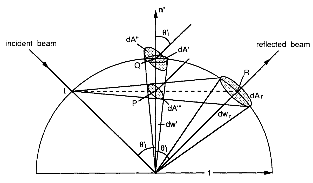
d\omega' = \frac{d\omega_r}{4\cos{\theta_i'}}
$$
$$
d\omega' = \frac{d\omega_r}{4\cos{\theta_i'}}
$$