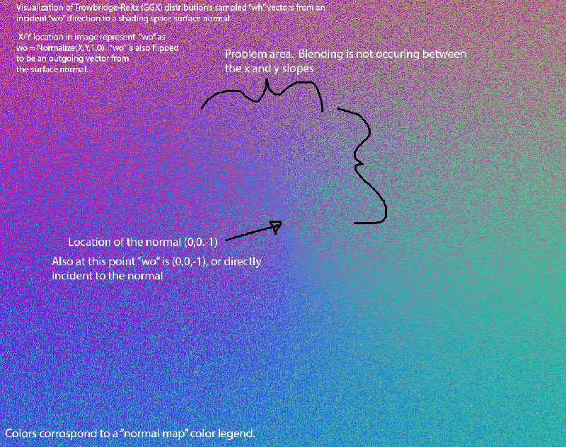
I am attempting to visualize the raw output from PBRT's half-vector sampling function, based on the trowbridge-reitz distribution. I'm isolating only the distribution and the associated functions necessary to sample it.
The function is based on the standard GGX half vector sampling formula:
$$\theta_s = arctan(\frac{\alpha_g\sqrt{\xi_1}}{\sqrt{1-\xi_1}})$$ $$\phi_s = 2\pi\xi_2$$
(from Walter GGX: http://www.cs.cornell.edu/~srm/publications/EGSR07-btdf.pdf)
but the PBRT version has a lot more black magic related to importance sampling only directions that make significant contributions based on the incoming "wo" angle. That one detail is making it hard for me to find published papers which specify how to add this directional importance sampling to the standard GGX sampling function.
Anyway, these angles come back from the sampling function as a vector 3 and spherical coordinates with $$Normalize([\theta_s,\phi_s, 1.0])$$ which should perturb the surface normal, creating the half vector to reflect around.
At this point I am only trying to make sense of the output from the "sample wh" function. To visualize the results (raw "wh" output) I made a little graphics utility to output the results to a "normal map". Here is the output:
And a live webgl example here that continually runs new random numbers through the output (as if monte carlo sampling were running): http://rdtests.ml3ds-test.com/microfacettesting.html
My expectation of the output would be a somewhat smooth gradient blend of the wh orientations as the x and y slopes cross into each other. But what i'm seeing is an area between the 2 axes that doesn't want to blend well. The random noise is good/expected, but you can see that inside the x/y blend areas, even the noise becomes fairly non-random.
Can anyone give me some tips on what the half vector sampling should graph like, or some pointers to papers/published work that I can use to locate test data, graphs, or other educational material that could help me figure this out?
