How to properly use the BRDF from glTF 2.0 specification in path tracing while using metallic/roughness materials?

Question

I've built a renderer which should render glTF materials, as they are defined in their specification. So I should be able to render satisfying (similar to Cycles and Ospray) results just from the base color, metallic and roughness factors. I've implemented their suggested BRDF, but I'm afraid I'm using it wrong, or I'm making a mistake somewhere else.

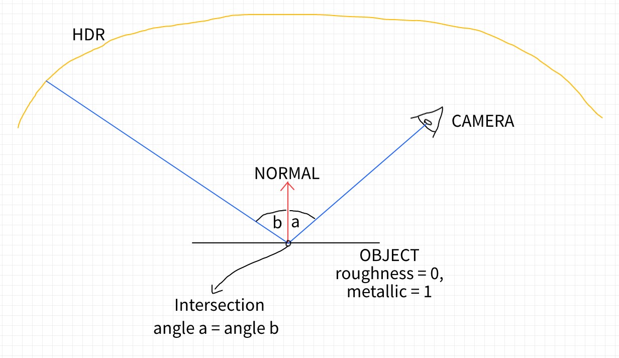
I'll now describe the steps in my renderer, using the simplest example: light is given by an HDR background and there is one object in the scene with roughness = 0 and metallic = 1. I've also attached a sketch of what I'm talking about so it's easier to follow.

Steps in bouncing:

1. Ray is shot from the camera
2. Ray hits object
3. Ray bounces in a mirror-like fashion because of the mentioned material properties
4. Ray hits HDR (hit on the HDR = miss all other objects)
5. Path ends

Reporting works like this:

1. I have the entire path with all three points (HDR, object, camera).
2. I start from the HDR and assign the path RGB values to the RGB values at the sampled point on the HDR. For example, path.RGB = (0.2, 0.8, 0.9).
3. I continue along the path and come to the point on the object. From the intersection data I get all the necessary information (base color, metallic, roughness and the normal at that point).
4. I provide all that info to the BRDF function and it returns some RGB values.
5. I multiply the RGB values which I got from the BRDF with the current path RGB (which is just the HDR values at this point) and that becomes the new path RGB.
6. I get to the camera point, and save the path RGB for writing to image later.

I simplified some parts which I'm fairly certain are not the cause of the problem, like the distance dependency and sampling and stuff like that.

So to get to the actual problem,

at the second point on the path (object intersection), my light vector is pointing towards the point on the HDR and my view vector is pointing towards the camera. Since the roughness at this point is 0, these two vectors are mirror images of one another, around the normal vector. So their half vector is the same vector as the normal vector. And when H (half vector) and N (normal vector) are the same, the BRDF produces a specular highlight, that happens because the D term (Trowbridge-Reitz/GGX microfacet distribution) ends up as a ridiculously large value. Now I'm aware that this should happen, If I were to use a point light source instead of the HDR, I would get the appropriate specular highlight, but that's because the light vector in that case is defined by the position of point light, and only a few points on the surface would fulfill the condition where H and N are the same (or no rays would in case of no roughness and point light with no radius). Problem appears when the light direction is the next point on the path since the direction towards it is the perfect reflection of the incident ray.

In the image I've attached, all rays hitting the object would bounce mirror-like, and each point on the object would be considered a specular highlight by the BRDF and it would return RGB values which go up to 8e14. By multiplying the path.RGB with those values, I would break the energy conservation, so currently I normalize them, but that also leads to problems. Black objects report with values around 5e10, and white objects as 8e14, as mentioned. Both end up normalized to (1, 1, 1) and look the same, even though they're opposites.

Now I'm not sure where exactly I'm I making a mistake, I've had my implementation of the BRDF checked multiple times, it's exactly like the specification.

Is my mistake considering the light vector to be the next (or previous, depends where you start from) point on the path? Or is it something else?

Answer 1

In rendering, we want to integrate over the light paths (with Monte Carlo integration). The common simplification is that the emissive surfaces emit radiance and the camera is sensitive to radiance, so the game becomes integrating radiance. Whereas, it looks like you're just tracing rays and multiplying stuff together.

Intuitively, let's suppose you have a very specular BRDF. For any particular incident ray, the value of the BRDF within the lobe is high, but the solid angle of the lobe itself is small. This is the part you're not accounting for, the integration domain.

---

Recall the rendering equation, and notice that it's an integral: $$ L(x,\omega_o) = \int_\Omega L(x,\omega_i) ~ ( n \cdot \omega_i ) ~ f_r(\omega_i,x,\omega_o) ~ d \omega_i $$ The Monte Carlo integration for this is what we expect: take a sample from the integrand and divide by the probability density of choosing it. Averaging a bunch of such calculations produces the same thing in expectation: $$ L(x,\omega_o) = E\left[ \frac{1}{N}\sum_{k=1}^N \frac{L(x,\omega_k) ~ ( n \cdot \omega_k ) ~ f_r(\omega_k,x,\omega_o) }{\text{pdf}(\omega_k)} \right]\\ \hspace{5cm}\text{where each }\omega_k\text{ sampled from }\Omega\text{ according}\\ \hspace{5.3cm}\text{to a distribution characterized by }\text{pdf}(\omega_k) $$ That averaging step is generally done in the main loop (averaging a bunch of paths instead of individual surface interactions), so the Monte Carlo estimator for a single surface interaction is just: $$ L(x,\omega_o) ~~\sim~~ L(x,\omega_k) ~ ( n \cdot \omega_k ) ~ f_r(\omega_k,x,\omega_o) ~/~ \text{pdf}(\omega_k) $$ I reckon the proximate problem is that you're missing that division.

The $\text{pdf}(\omega_k)$ term is the probability density of sampling your ray. For example, if you choose rays uniformly at random, then the probability density is just the total probability ($1$) divided by the integration domain ($\Omega$, the surface area of the hemisphere, $2\pi$). That is, $\text{pdf}(\omega_k)=1/(2\pi)$: $$ L(x,\omega_o) ~~\sim~~ L(x,\omega_k) ~ ( n \cdot \omega_k ) ~ f_r(\omega_k,x,\omega_o) ~/~ (1/(2\pi))\\ \hspace{5cm}\text{when }\omega_k\text{ sampled uniformly from }\Omega $$

Now, sampling uniformly from the hemisphere is a terrible way to sample essentially every BRDF. A slightly more complicated way is to sample proportional to the cosine-weighted hemisphere—i.e., $\text{pdf}(\omega_k)=( n \cdot \omega_k )/\pi$: $$ L(x,\omega_o) ~~\sim~~ L(x,\omega_k) ~ ( n \cdot \omega_k ) ~ f_r(\omega_k,x,\omega_o) ~/~ (( n \cdot \omega_k )/\pi)\\ \hspace{5cm}\text{when }\omega_k\text{ sampled cosine-weighted from }\Omega $$ This is much better for most BRDFs (in fact it's optimal for a Lambertian BRDF, because it exactly matches it). It's still pretty bad for most BRDFs, but it's a reasonable "default" sampler if you have no idea what the BRDF looks like or you're just testing.

You can freely choose how you sample rays, but you must always account for that sampling technique by dividing out its probability density.

In this case, you mentioned sampling in "a mirror-like fashion", which could mean anything, and you're working with a microfacet BRDF, which is nontrivial. Sampling these more complicated BRDFs is difficult, but there are resources available, and you can always use a simpler sampler (e.g. cosine-weight sampling) and it will still work (the integral estimate will just converge slower).

---

P.S.: for testing purposes, I recommend you get this working for a Lambertian BRDF with the uniformly random sampler. Then upgrade to the cosine-weighted sampler. Then add the microfacet BRDF. Then work on more advanced samplers for the microfacet BRDF.

P.P.S.: I strongly recommend doing a "white furnace test" for each test. You render a plane with albedo 1 inside of a flat-gray environment map. If everything is working correctly, the plane will converge to exactly the same color as the background and "disappear".