How to find the major and minor axes of a convex hull?

Question

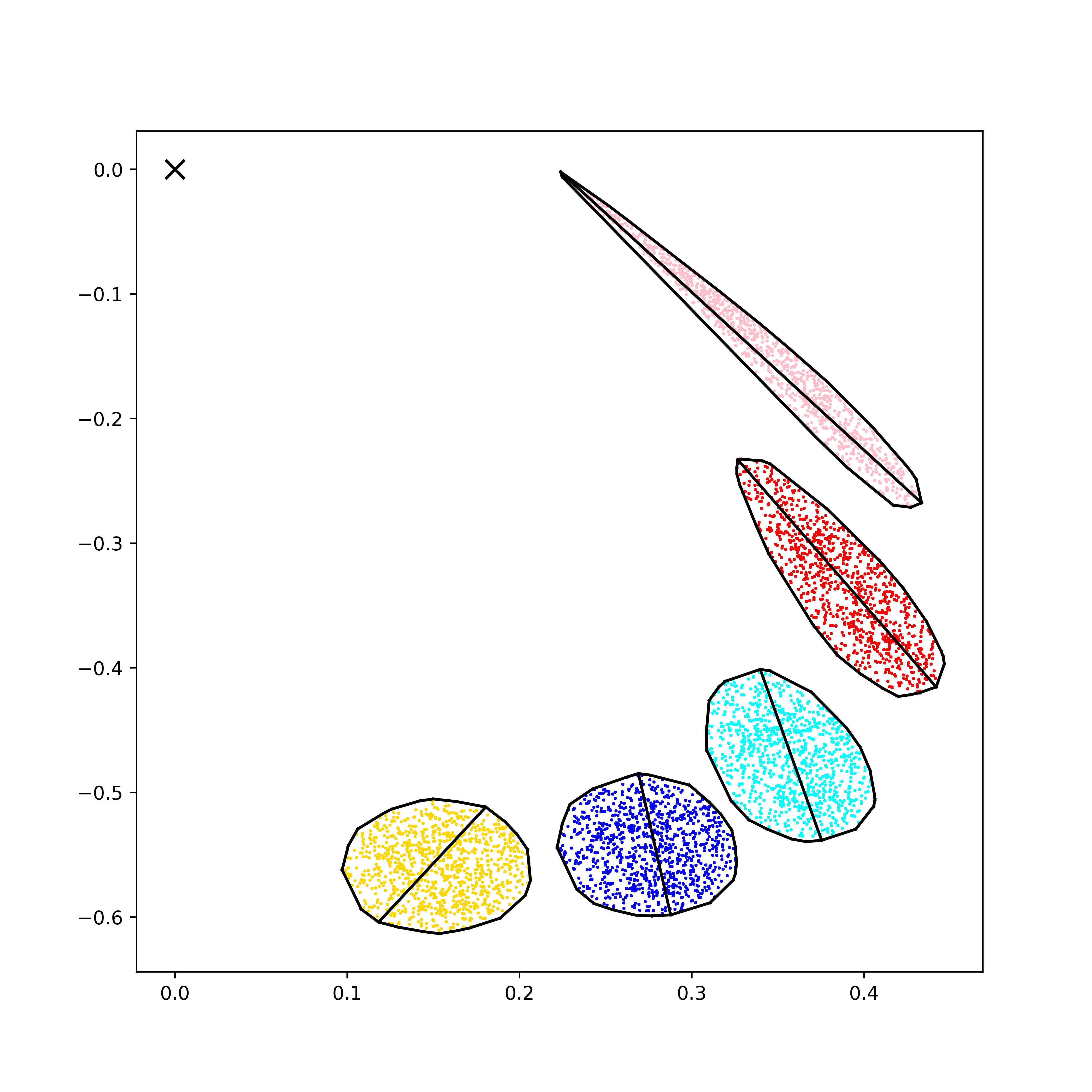
I have a set of particles in a gravitationally bound system. The shape of the particles change with time, I have used a convex hull algorithm to "enclose" the particles of the cloud. I want to find the major and the minor axes of the cloud.

hulls = [hull1, hull2, hull3, hull4, hull5]

for hull in hulls:
    for simplex in hull.simplices:
        plt.plot(hull.points[simplex, 0], hull.points[simplex, 1], '-', color='black')
    
    points = hull.points[hull.vertices] # shape: (#vertices, #coordinates)
    max_distance = 0
    major_axis = None
    for i in range(len(points)):
        for j in range(i + 1, len(points)):
            distance = np.linalg.norm(points[i] - points[j])
            if distance > max_distance:
                max_distance = distance
                major_axis = (points[i], points[j])

    plt.plot([major_axis[0][0], major_axis[1][0]], [major_axis[0][1], major_axis[1][1]], color='black')

The plot shows the cloud changing with time. Each cloud is for a different time.

I have been able to get the major axes from this. But not the minor axes. How can I do it? Basically just need the distance of the perpendicular through the middle of the major axis. This is a aspect ratio problem. I need the length and width of the cloud. If there is a better way to do this, please let me know.

Answer 1

I think we can compute an inertia-like term of the cloud, the eigenvectors will tell us the two (major and minor) axes in 2D, and the eigenvalues will tell us the extents along the two axes. This is probably the "PCA idea" mentioned by lhf in the comments.

I tried this idea out in Matlab. The code should work fine in Octave too.

First seed some points in an ellipse with scaling/rotation/translation. In your case you should use the real inputs. I only use this for testing.

function [X,Y] = sample(a, b, s, q, tx, ty, n)
    X = (rand(n, 1) - 0.5) * s;
    Y = (rand(n, 1) - 0.5) * s;
    X2 = X .* X / (a * a);
    Y2 = Y .* Y / (b * b);
    i = (X2 + Y2) < 1;
    X0 = X(i);
    Y0 = Y(i);
    X = cos(q) * X0 - sin(q) * Y0 + tx;
    Y = sin(q) * X0 + cos(q) * Y0 + ty;
end

On my side, I did this to generate the cloud: (also take the total number of points)

[X,Y]=sample(2,1,4,pi/6, 1.9, 4.7,2000);
N=size(X)
N=N(1)

Then compute the center of the points and normalize the inputs:

C=[sum(X)/N, sum(Y)/N];
nX=X-C(1);
nY=Y-C(2);

I will compute the inertia-like term using nX and nY. Given a vector $\mathbf{r}$, each inertia term is $\mathbf{I} \mathbf{r}^T \mathbf{r} - \mathbf{r} \mathbf{r}^T$. Here $\mathbf{I}$ is the identity matrix. In Matlab/Octave:

function M = ptinertia2(X, Y)
    rtr = (X' * X + Y' * Y) * eye(2);
    P = [X, Y];
    rrt = P' * P;
    M = rtr - rrt;
end

The inertia and its eigen pairs are:

M=ptinertia2(nX,nY);
[V,D]=eig(M)
f=sqrt(D(2,2)/D(1,1))

(f is the scaling factor on the major axis).

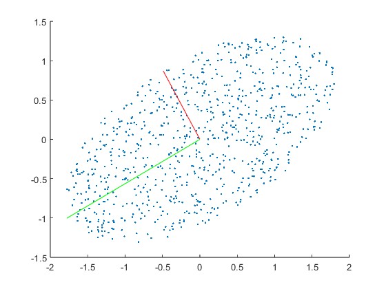
The eigenvalues are in the diagonal matrix D, and the eigenvectors are in the orthonormal matrix V. To visualize the inputs and the identified axes:

scatter(nX,nY,'.')
hold on
line([0, V(1,2)],[0,V(2,2)],'Color','red')
line([0, V(1,1)*f],[0,V(2,1)*f],'Color','green')