3
$\begingroup$

I asked a similar question here before but since the previous post original question was different, I think it was confusing people. So I've voted to close that and asking the new question here. I'm doing a volume rendering project and made a cubic spline editor for transfer function. I used this as a source which basically uses Wolfram as the main source. Now Wolfram defines a parametric representation. After I made it, I tried to compare it online but the curves are different. The only difference I found is that the online version is using a non-parametric representation.

Here's mine. enter image description here

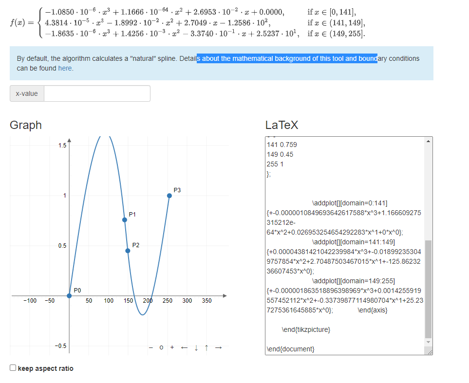
And here's the online version enter image description here

In order to clarify a bit more on what I'm trying to do. I have 2 variables.

$X = [0, 255] $

$Y = [0, 1] $

For every given $X$ value I need the interpolated $Y$ value. At first glance it seems that the explicit form of cubic spline is what I want. But I have another case where $Y$ values are RGB triplets $(r,g,b)$. Since the parametric representation doesn't have to deal with dimensions and since the code was already online I'm using the parametric form. The parametric form uses the parameter $t \in [0,1]$ for every segment.

Now things get a little trickier. Technichally my graph is of $(t, Y(t))$ but as you can see in the first picture the X-axis isn't $t$ but the previously defined $X$ which is in range $[0-255]$. I'm simply rescaling between $X$ and $t$. So if I get $t = 0.5$ for the first segment as an example, I'd take the two bounding control points which resolve to $(0,0)$ and $(141, 0.759)$ in the first picture. Then do simple rescaling like

$0 + (141 - 0) * t$

to get my iso-value and plot the graph. Here's how I'm actually drawing the graph

float t_step = 1/255.0f;
for(int i = 0; i < knots.size() - 1; i++)
  {
    for (int i_step = 1; i_step <= num_line_segments; i_step++)
    {
        glm::vec2 coord;
        coord.x = knots[i].iso_value + (t_step * i_step * (knots[i+1].iso_value - knots[i].iso_value));
        coord.y = glm::clamp(alpha_spline.getPointOnSpline(t_step * i_step, i).w, v_min.y, v_max.y);
        win->DrawList->_Path.push_back(getAbsMousePositionFromPoint(coord) );
    }
  }
  
getAbsMousePositionFromPoint(glm::vec2 v)
{
  glm::vec2 v_min(0,0), v_max(255, 1.0)
  glm::vec2 t = (v - v_min) / (v_max - v_min);
  return glm::mix(graph_bot_left, graph_top_right, t);   // both "graph_bot_left" and "graph_top_right" are absolute coordinates of the drawing region
}

Basically I need absolute coordinates for drawing anything on the screen. Each segment of the spline is basically drawn as a polyline. Just to be on the safe side I have currently set the number of line segments per curve of the spline to be 255. This means per segment of the spline I need to draw 255 line segments. I step along t then transform it to the proper X-value by doing the transformation step as I told above then find absolute coordinates from that X-value and draw the segment there.

Now all I wanna know is, do parametric and explicit forms give different curves? If not, then is there something wrong with the rescaling step I'm doing above or something else?

P.S :- I've checked the formulation and the boundary conditions of the online one and all are similar to the Wolfram one. Both mine and the online one are natural cubic splines. I've also double checked my code, even derived the whole parametric form on paper and checked the code with the one derived on paper and it matches perfectly so I'm pretty sure the code isn't wrong. Still here's my spline source as a reference if anybody here knows programming

UPDATE:- So I just found another guy using the same logic as well here. I guess the math is all right then. Don't see where's the problem then.

$\endgroup$
5
  • $\begingroup$ The implicit and parametric forms are equivalent by definition. So the curves should look virtually identical. Are the coefficients reversed in the code? Usually the equation is $a^3t+b^2t+ct+d$ which would be $(((a * time) + b) * time + c) * time + d;$ but the linked coded seems to have $d^3t+c^2t+bt+a$ which is translated to $a + t * (b + t * (c + t * d))$ $\endgroup$
    – pmw1234
    Commented Aug 24, 2021 at 13:36
  • $\begingroup$ @pmw1234 - Yea I seemed to have missed this point. The Wolfram and the code give the last equation that is $a + bt + ct^2 + dt^3$ where as the online has $ax^3 + bx^2 + cx + d$. But I don't think its making any difference because then in the online version the coeffecient $a$ and $b$ are actually $d$ and $c$ in my code respectively. Here's the link to the online just in case. Also added in OP. timodenk.com/blog/cubic-spline-interpolation $\endgroup$ Commented Aug 24, 2021 at 16:31
  • 1
    $\begingroup$ If you're talking about defining y as a cubic function of x directly, versus defining x and y both as cubic functions of a parameter t, then yes those are totally different things and will behave differently. The former is a 1D spline and the latter is a 2D spline. $\endgroup$ Commented Aug 24, 2021 at 18:47
  • $\begingroup$ But if you're just talking about a 1D spline and rescaling the parameter (t = x/255) then that shouldn't make any difference as long as you are doing the rescaling correctly. $\endgroup$ Commented Aug 24, 2021 at 18:50
  • $\begingroup$ @NathanReed - Yes, I'm talking about the latter one (1D spline). Simply speaking I could have defined $Y(x)$ and gotten my interpolated values as a function of $x$ but I chose to do $Y(t)$ then rescale $x$ to $t$ and vice versa as mentioned above. But I'm still getting different results and I dunno why. $\endgroup$ Commented Aug 25, 2021 at 9:29

1 Answer 1

1
+100
$\begingroup$

The two graphs are graphing Cubic Splines but they are not equivalent splines. The method used in the code you linked produces a curve that is very local to the points and produces the tightest fit to a data set of any of the curves. This curve is only affect by adjacent (knots) control points.

The method used in the online calculator produces a similar curve but individual segments are affected by control points that are up to 2 positions away which change the tangent and causes the big dips in the curve shown in the graph.

You should be able to convince yourself of this by looking at the two matrices used in the solution for both curves. The tridiagonal matrix can only affect adjacent rows and columns where as the matrix shown in the solution for the online calculator effects several rows and columns, this translates to very different curves.

I attempted to use Mathematica to check the curve produced by the linked code but the resulting curve (as described by the wolfram math web link in the references you gave) was not even a cubic spline.

I was able to verify the curve output by the online calculator in the web link using Maple, they both produce almost identical equations. MatLab supposedly has a function that will produce the same spline linked in your code but I don't have access to that program so wasn't able to verify it.

I started to convert the equations between implicit/explicit/parametric forms but that turned into more math then I am willing to do (and I didn't want to post a massive list of equations showing the conversion). But these are not implicit vs parametric forms of the same curve anyway so it would have been kind of pointless.

After all that I decided to implement my own version of the spline solver from the book wolfram references. ( I managed to get a used copy on the cheap ) My solution ended up being very similar to the code you linked and produced very similar results. The curves were slightly smoother at the control points but I think that I was using a different method of computing the values...along the lines of:

segment_count = knot_count -1;
vec4 solved_coefficients[segment_count];
vec2 curve[segment_count *100];
for each segment_count
  vec4 coeff = solved_coefficients[segment];
  for x=0 x<100; x++;
     t = 1.0/x;
     curve[knot*x] = calcPointOnLine( coeff, t);

This turned out to be a fun little side project into the different versions of fitted cubic splines.

Edit: The problem is that the terminology used to describe the splines is used so interchangeably that the different solutions which produce very different splines are given the same names. I found one paper which used the name "Cubic Hermite Spline" for the what we implemented, and it gave the name "Cubic Spline" for what the online calculator implemented.

It is also possible to make the splines equivalent to each other by playing with the knot positions. I refitted the Cubic spline to a Cubic Hermite by moving/adding knot positions separated by a distance of 1 and got exactly the same splines from both solutions. The other direction (which I didn't try) is to fit the cubic Hermite spline to the cubic spline by changing the knot sequence from 0,1,2,3 to 0,141,149,255.

When it is all said and done I think it is more about what kind of fit works best for your algorithm.

$\endgroup$
5
  • $\begingroup$ Dang bro, that's one heck of an effort. So in the end, this means the implementation is alright. But we still don't know what this implementation actually represents? I think it's a cubic spline but as you said it's different in the sense where only the adjacent knots affect the segment. I still don't get why or how parametric or implicit forms can produce this difference i.e. parameteric form produces a spline where the only adjacent knots affect the curve where as in implicit a small change in a knot can affect more than the adjacent knots. $\endgroup$ Commented Sep 26, 2021 at 15:08
  • $\begingroup$ The only thing the two solutions have in common is the fact that they pass through the set of points and are both cubic. They are very different ways of fitting a cubic curve to a set of points and the fact that one produces a parametric equation while the other produces an explicit solution is just a side effect of the approach used. (oh and I added an edit) $\endgroup$
    – pmw1234
    Commented Sep 26, 2021 at 23:41
  • 1
    $\begingroup$ Oh, one more little detail is the wolfram solution avoids Runge's Phenomenon better then any other approach so it is possible to use an algorithm that can reduce it sample points to a minimum number and still get reasonably accurate results. $\endgroup$
    – pmw1234
    Commented Sep 26, 2021 at 23:47
  • $\begingroup$ This cleared up many details. Thanks for the effort mate, much appreciated. $\endgroup$ Commented Sep 27, 2021 at 6:45
  • $\begingroup$ I just bumbled across this web page which is yet another way to compute the spline, it also discusses 1d vs 2d vs 3d, there are links to demos at the bottom of the page to :blog.demofox.org/2015/08/08/cubic-hermite-interpolation $\endgroup$
    – pmw1234
    Commented Sep 27, 2021 at 10:41

Your Answer

By clicking “Post Your Answer”, you agree to our terms of service and acknowledge you have read our privacy policy.

Not the answer you're looking for? Browse other questions tagged or ask your own question.